kakakakakku blog

Weekly Tech Blog: Keep on Learning!

scikit-learn の Pipeline を使って前処理やアルゴリズムをまとめて宣言する

scikit-learnPipeline を使うと,データセットの前処理や機械学習アルゴリズムなどを「1つのオブジェクトに」まとめることができる.

scikit-learn.org

前回の記事で紹介した「Kaggle Courses」「Intermediate Machine Learning」コースでも使われていたこともあり,もう少しドキュメントを読みながら試していく.

kakakakakku.hatenablog.com

Pipeline に入門する

「Kaggle Courses」のコースを参考にサンプルコードを書くと,以下のようになる(重要なコードのみを抜粋している).Pipeline を使わずにコードを書くと SimpleImputerOneHotEncoderRandomForestRegressor など,それぞれで fit()fit_transform() を実行する必要があるため,コード量を減らしつつ,可読性が高く実装できる.イイネ👏

from sklearn.ensemble import RandomForestRegressor
from sklearn.impute import SimpleImputer
from sklearn.pipeline import Pipeline
from sklearn.preprocessing import OneHotEncoder

X_train, X_test, y_train, y_test = train_test_split(X, y, train_size=0.8, test_size=0.2, random_state=0)

pipeline = Pipeline(
    steps=[
        ('imputer', SimpleImputer(strategy='most_frequent')),
        ('encoder', OneHotEncoder(handle_unknown='ignore')),
        ('model', RandomForestRegressor(n_estimators=50, random_state=0))
    ]
)

pipeline.fit(X_train, y_train)

pipeline.predict(X_test)

また Pipelineverbose=True パラメータを追加すると fit() を実行しながら以下のように進捗を表示することもできる.

pipeline = Pipeline(
    steps=[
        ('imputer', SimpleImputer(strategy='most_frequent')),
        ('encoder', OneHotEncoder(handle_unknown='ignore')),
        ('model', RandomForestRegressor(n_estimators=50, random_state=0))
    ],
    verbose=True
)

# [Pipeline] ........... (step 1 of 3) Processing imputer, total=   0.1s
# [Pipeline] ........... (step 2 of 3) Processing encoder, total=   0.1s
# [Pipeline] ............. (step 3 of 3) Processing model, total=  10.1s

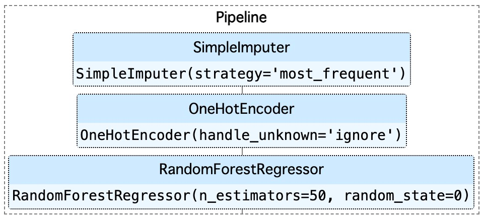
そして,以下のドキュメントを参考に set_config() を使って「ダイアグラム表示」を有効化すると,以下のように Pipeline 構成を図として表示できる.実際には枠をクリックすることができて,パラメータを表示したり,非表示にしたりできる.

scikit-learn.org

from sklearn import set_config
set_config(display='diagram')
pipeline

f:id:kakku22:20211123175045p:plain

Pipeline で前処理をカテゴライズする

さらに Pipeline の中で前処理をカテゴライズすることもできる.例えば,以下のように numeric_preprocessor(量的変数)categorical_preprocessor(カテゴリ変数) としてまとめている(重要なコードのみを抜粋している).最終的には make_pipeline() を使って RandomForestRegressor とまとめている.今回のサンプルコード以上に前処理などが多いときに効果が出そう.

scikit-learn.org

from sklearn.compose import ColumnTransformer
from sklearn.ensemble import RandomForestRegressor
from sklearn.impute import SimpleImputer
from sklearn.pipeline import make_pipeline
from sklearn.pipeline import Pipeline
from sklearn.preprocessing import OneHotEncoder, StandardScaler

numeric_preprocessor = Pipeline(
    steps=[
        ('imputer', SimpleImputer(strategy='most_frequent')),
        ('scaler', StandardScaler()),
    ]
)

categorical_preprocessor = Pipeline(
    steps=[
        ('onehot', OneHotEncoder(handle_unknown='ignore')),
    ]
)

pipeline = make_pipeline(
    ColumnTransformer(
        [
            ('numerical', numeric_preprocessor, numerical_cols),
            ('categorical', categorical_preprocessor, categorical_cols)
        ]
    ),
    RandomForestRegressor(n_estimators=50, random_state=0)
)

同じく set_config() を使って「ダイアグラム表示」を有効化すると,より整理された Pipeline 構成を表示することができた.

from sklearn import set_config
set_config(display='diagram')
pipeline

f:id:kakku22:20211124095951p:plain

まとめ

scikit-learnPipeline を使うと,データセットの前処理や機械学習アルゴリズムなどを「1つのオブジェクトに」まとめることができる.今回はシンプルな Pipeline 構成とカテゴライズをした構成を紹介した.ドキュメントを読むと,他にも GridSearchCV と組み合わせてハイパーパラメータを探索することもできて,便利だった.

scikit-learn.org

Intermediate Machine Learning : Kaggle Courses で学びながら「住宅価格予測」コンペに参加する

Kaggle が公開している「Kaggle Courses」「Intermediate Machine Learning」コースを受講した.Kaggle のコンペティション「Housing Prices Competition for Kaggle Learn Users(住宅価格予測)」をテーマに試行錯誤をして,実際にモデルを登録することもできる.アルゴリズムとしては「ランダムフォレスト」「XGBoost」を使う.アジェンダを見るとわかる通り,データセットの前処理からモデルの構築評価まで幅広く体験できる.

www.kaggle.com

なお,前提コースである「Pandas」「Intro to Machine Learning」は既に受講していて,以下にまとめてある.

kakakakakku.hatenablog.com

kakakakakku.hatenablog.com

アジェンダ 🏠

「Intermediate Machine Learning」コースには「計7種類」のレッスン(ドキュメントと演習)がある.

  1. Introduction
  2. Missing Values
  3. Categorical Variables
  4. Pipelines
  5. Cross-Validation
  6. XGBoost
  7. Data Leakage

住宅価格予測 🏠

1460 件のデータセットに 80 個の特徴量を含んでいる.その中から今回は 7 個の特徴量を使う.このあたりは前提コース「Intro to Machine Learning」と同じ.そして,特徴量の中に予測する SalePrice(住宅価格) も含まれていることから「教師あり学習(回帰)」と言える.

X_full.shape
# (1460, 80)

X.shape
# (1460, 7)

X.columns
# Index(['LotArea', 'YearBuilt', '1stFlrSF', '2ndFlrSF', 'FullBath', 'BedroomAbvGr', 'TotRmsAbvGrd'], dtype='object')

まず 1. Introduction2. Missing Values3. Categorical Variables4. Pipelines では,scikit-learnRandomForestRegressor を使って「ランダムフォレスト」でモデルを構築する.以下のように適当にパラメータを設定して比較したり(今回は model_3 の平均絶対誤差 MAE が1番低かった👌),欠損値を考慮したり,カテゴリ変数をエンコーディングしたり,一歩一歩モデル精度を向上させていく.また scikit-learnPipeline を使って,コード実装を改善する.

model_1 = RandomForestRegressor(n_estimators=50, random_state=0)
model_2 = RandomForestRegressor(n_estimators=100, random_state=0)
model_3 = RandomForestRegressor(n_estimators=100, criterion='mae', random_state=0)
model_4 = RandomForestRegressor(n_estimators=200, min_samples_split=20, random_state=0)
model_5 = RandomForestRegressor(n_estimators=100, max_depth=7, random_state=0)

実際に評価をしながら進めるため,今回は欠損値を平均値で埋めるよりも特徴量を削除した方がパフォーマンスが良いなど,予想とは違う気付きもあって良かった.

  • Missing Values(欠損値)
    • [1] A Simple Option: Drop Columns with Missing Values(単純に特徴量を削除する)
    • [2] A Better Option: Imputation(より良く平均値などで埋める)
    • [3] An Extension To Imputation(値を埋めつつ欠損値の有無を表現する新しい特徴量を追加する)
  • Categorical Variables(カテゴリ変数)
    • [1] Drop Categorical Variables(カテゴリ変数を削除する)
    • [2] Ordinal Encoding(順序エンコーディング)
    • [3] One-Hot Encoding(ワンホットエンコーディング)

実際に Kaggle コンペティションにモデルを登録して,Leaderboard で順位が上がっていくことも確認する🏆

f:id:kakku22:20211123120838p:plain

交差検証 🏠

5. Cross-Validation では,scikit-learncross_val_score() を使って「交差検証」を行う.分割数 cv35 に設定しながら最終的な平均値を確認する.

scikit-learn.org

そして「ランダムフォレスト」に設定するパラメータ n_estimators の最善値を探す.今回は n_estimators = 50, 100, 150, 200, 250, 300, 350, 400 で比較して,結果的として 200 のパフォーマンスが1番良かった.

f:id:kakku22:20211123122155p:plain

XGBoost 🏠

ここまでは「ランダムフォレスト(アンサンブル学習)」を使ってきたけど,次は「XGBoost(勾配ブースティング)」を適用する.以下のようにパラメータを変えて比較をするけど,重要なのはアルゴリズムを変えることも考えながらコンペティションに参加するという点になる.

my_model_1 = XGBRegressor(random_state=0)
# Mean Absolute Error: 17662.736729452055

my_model_2 = XGBRegressor(n_estimators=1000, learning_rate=0.05)
# Mean Absolute Error: 16688.691513270547

my_model_3 = XGBRegressor(n_estimators=1)
# Mean Absolute Error: 127895.0828807256

xgboost.readthedocs.io

Data Leakage 🏠

7. Data Leakage では,モデルに対する考察として「Data Leakage(データ漏洩)」を学ぶ.「Data Leakage」とは,トレーニングデータセットにターゲットに関する「含まれていはいけないデータが含まれていること」と言える.よって,モデルの検証時にはパフォーマンスが高くなり,本番環境にデプロイするとパフォーマンスが低くなってしまう.「Data Leakage」として,具体的には以下の2種類が載っていた.

  • Target leakage(ターゲット漏洩)
    • 例 : 肺炎予測をするときに「抗生物質を服用しているか」という特徴量を使ってしまう
      • 本来は「肺炎である」と診断されてから処方されるため,将来の予測には使えない
  • Train-Test Contamination(トレインテスト汚染)
    • 例 : データセットを前処理する場合に欠損値を平均値などで埋める場合に検証データの精度が高くなってしまう
      • 検証データを除外して前処理をする
      • scikit-learntrain_test_split() から Train-Test という名前になっている

まとめ 🏠

「Kaggle Courses」「Intermediate Machine Learning」コースを受講した.Kaggle のコンペティション「Housing Prices Competition for Kaggle Learn Users(住宅価格予測)」に参加することもできて,一般的な機械学習ワークフローを体験することができた.とても良かった👏

次は「Feature Engineering」コースと「Machine Learning Explainability」コースに進もうと思う.

f:id:kakku22:20211123123758p:plain

imbalanced-learn の SMOTE モジュールを使って簡単にオーバーサンプリングを実現する

分類などの機械学習モデルを構築するときにデータセットに偏り(不均衡データ)があると適切に学習できない可能性がある.データセットを強制的に増やす操作を「オーバーサンプリング」と言って,SMOTE (Synthetic Minority Over-sampling Technique)ADASYN (Adaptive Synthetic) など,具体的な「オーバーサンプリング手法」がよく知られている.ちなみに SMOTEk-NN (k-Nearest Neighbor) : k近傍法 を参考に近接データを増やす.

imbalanced-learn とは

今回紹介する imbalanced-learn「不均衡データ」を扱うライブラリで「オーバーサンプリング」「アンダーサンプリング」などを簡単に実装できる.そして scikit-learn と互換がある.また GitHub だと scikit-learn-contrib プロジェクトで管理されている.

github.com

SMOTE モジュールを試す

今回は imbalanced-learn に入門するために SMOTE モジュールを試す.Over-sampling のドキュメントに載っているサンプルコードを参考にしつつ,もっと簡単に書き直してみた.

まず,scikit-learnmake_classification() 関数を使って,2000 データセットを 0.05 : 0.95 の割合で不均衡データとして生成した.特徴量はシンプルに2個にした.そして imbalanced-learnSMOTE モジュールで fit_resample() 関数を使うと簡単に「オーバーサンプリング」をすることができる.

from imblearn import FunctionSampler
from imblearn.over_sampling import SMOTE
from sklearn.datasets import make_classification
import matplotlib.pyplot as plt

def plot_resampling(X, y, sampler, ax):
    X_res, y_res = sampler.fit_resample(X, y)
    ax.scatter(X_res[:, 0], X_res[:, 1], c=y_res, alpha=0.8, edgecolor="k")
    title = f"Resampling with {sampler.__class__.__name__}"
    ax.set_title(title)

X, y = make_classification(
    n_samples=2000,
    n_features=2,
    n_informative=2,
    n_redundant=0,
    n_classes=2,
    weights=[0.05, 0.95],
    class_sep=1.0,
    random_state=1
)

fig, axs = plt.subplots(nrows=2, ncols=1, figsize=(20, 20))

samplers = [
    FunctionSampler(),
    SMOTE()
]

for ax, sampler in zip(axs.ravel(), samplers):
    plot_resampling(X, y, sampler, ax)

そして matplotlibscatter() 関数で散布図を描画した.Resampling with FunctionSampler(通常)Resampling with SMOTE(オーバーサンプリング) を比較すると,特徴量(紫色)に大きく差を確認できる.便利だ!

f:id:kakku22:20211101135838p:plain

関連記事

kakakakakku.hatenablog.com

kakakakakku.hatenablog.com

iris データセットを libsvm フォーマットにする : scikit-learn の dump_svmlight_file()

scikit-learndatasets モジュールの中に libsvm フォーマットのデータセットを扱う関数がある.libsvm フォーマットは以下のフォーマットでデータセットを表現し,1番左にラベル(教師データ)を持つ.例えば Amazon SageMaker の組み込みアルゴリズム XGBoost でもサポートされている.

<label> <index1>:<value1> <index2>:<value2> ...

以下のサイトには libsvm フォーマットで多種多様なデータセットが公開されている.

www.csie.ntu.edu.tw

libsvm フォーマット例

例えば iris データセット(アヤメ)に以下のサンプルデータセットがあったとする.Label は3種類ある.

  • 0 = setosa(ヒオウギアヤメ)
  • 1 = versicolor(ハナショウブ)
  • 2 = virginica(カキツバタ)
sepal length (cm) sepal width (cm) petal length (cm) petal width (cm) Label
5.1 3.5 1.4 0.2 0
4.9 3.0 1.4 0.2 0
4.7 3.2 1.3 0.2 0

サンプルデータセットを libsvm フォーマットにすると以下となる.

0 0:5.1 1:3.5 2:1.4 3:0.2
0 0:4.9 1:3 2:1.4 3:0.2
0 0:4.7 1:3.2 2:1.3 3:0.2

scikit-learn dump_svmlight_file() 関数

scikit-learn を使って簡単に iris データセット(アヤメ)をセットアップできるため「特徴量」「ラベル」を取得して,同じく scikit-learndump_svmlight_file() 関数をさっそく試す.最終的に iris-libsvm ファイルに書き出す.コードはシンプルに書ける!

from sklearn.datasets import dump_svmlight_file
from sklearn.datasets import load_iris

iris = load_iris()

# 特徴量
x = iris.data

# ラベル
y = iris.target

dump_svmlight_file(x, y, 'iris-libsvm')

scikit-learn.org

実行後に head -n 50 iris-libsvm コマンドを実行して書き出した iris-libsvm ファイルを確認すると,期待通りに libsvm フォーマットになっていた.

0 0:5.1 1:3.5 2:1.4 3:0.2
0 0:4.9 1:3 2:1.4 3:0.2
0 0:4.7 1:3.2 2:1.3 3:0.2
0 0:4.6 1:3.1 2:1.5 3:0.2
0 0:5 1:3.6 2:1.4 3:0.2
0 0:5.4 1:3.9 2:1.7 3:0.4
0 0:4.6 1:3.4 2:1.4 3:0.3
0 0:5 1:3.4 2:1.5 3:0.2
0 0:4.4 1:2.9 2:1.4 3:0.2
0 0:4.9 1:3.1 2:1.5 3:0.1
0 0:5.4 1:3.7 2:1.5 3:0.2
0 0:4.8 1:3.4 2:1.6 3:0.2
0 0:4.8 1:3 2:1.4 3:0.1
0 0:4.3 1:3 2:1.1 3:0.1
0 0:5.8 1:4 2:1.2 3:0.2
0 0:5.7 1:4.4 2:1.5 3:0.4
0 0:5.4 1:3.9 2:1.3 3:0.4
0 0:5.1 1:3.5 2:1.4 3:0.3
0 0:5.7 1:3.8 2:1.7 3:0.3
0 0:5.1 1:3.8 2:1.5 3:0.3
0 0:5.4 1:3.4 2:1.7 3:0.2
0 0:5.1 1:3.7 2:1.5 3:0.4
0 0:4.6 1:3.6 2:1 3:0.2
0 0:5.1 1:3.3 2:1.7 3:0.5
0 0:4.8 1:3.4 2:1.9 3:0.2
0 0:5 1:3 2:1.6 3:0.2
0 0:5 1:3.4 2:1.6 3:0.4
0 0:5.2 1:3.5 2:1.5 3:0.2
0 0:5.2 1:3.4 2:1.4 3:0.2
0 0:4.7 1:3.2 2:1.6 3:0.2
0 0:4.8 1:3.1 2:1.6 3:0.2
0 0:5.4 1:3.4 2:1.5 3:0.4
0 0:5.2 1:4.1 2:1.5 3:0.1
0 0:5.5 1:4.2 2:1.4 3:0.2
0 0:4.9 1:3.1 2:1.5 3:0.2
0 0:5 1:3.2 2:1.2 3:0.2
0 0:5.5 1:3.5 2:1.3 3:0.2
0 0:4.9 1:3.6 2:1.4 3:0.1
0 0:4.4 1:3 2:1.3 3:0.2
0 0:5.1 1:3.4 2:1.5 3:0.2
0 0:5 1:3.5 2:1.3 3:0.3
0 0:4.5 1:2.3 2:1.3 3:0.3
0 0:4.4 1:3.2 2:1.3 3:0.2
0 0:5 1:3.5 2:1.6 3:0.6
0 0:5.1 1:3.8 2:1.9 3:0.4
0 0:4.8 1:3 2:1.4 3:0.3
0 0:5.1 1:3.8 2:1.6 3:0.2
0 0:4.6 1:3.2 2:1.4 3:0.2
0 0:5.3 1:3.7 2:1.5 3:0.2
0 0:5 1:3.3 2:1.4 3:0.2

関連記事

kakakakakku.hatenablog.com

Intro to Machine Learning : Kaggle Courses で「住宅価格予測」に入門した

Kaggle が公開している「Kaggle Courses」で機械学習に入門できる「Intro to Machine Learning」コースを受講した.Intro と書いてある通り,入門レベルではあるけど,scikit-learn を使って「決定木(回帰)」「ランダムフォレスト」「住宅価格予測」を体験できる.紹介も兼ねて,受講したメモを整理してまとめる!

www.kaggle.com

アジェンダ 🌴

「Intro to Machine Learning」コースには「計7種類」のレッスン(ドキュメントと演習)がある.なお,データを取り扱うときに Pandas の知識は最低限必要になるため,もし不安があれば,先に「Pandas」コースを受講しておくと良いと思う.詳細は前にブログで紹介した.

  1. How Models Work
  2. Basic Data Exploration
  3. Your First Machine Learning Model
  4. Model Validation
  5. Underfitting and Overfitting
  6. Random Forests
  7. Machine Learning Competitions

kakakakakku.hatenablog.com

1. How Models Work 🌴

最初は今回テーマとする「住宅価格予測」の概要と「決定木」の紹介が載っている.例えば「寝室を2つ以上持っているかどうか」という基準だと,一般的な傾向としては寝室が多い方が住宅価格は高いと予測できる.しかし,実際にはバスルームやロケーションなど,他にも様々な特徴を考慮する必要があり,それらを「決定木」として,木構造で Yes/No に分岐していく.

f:id:kakku22:20210616113341p:plain
How Models Work | Kaggle より引用

2. Basic Data Exploration 🌴

さっそく Pandas を使って「住宅データ」を確認していく.特に複雑な内容はなく,DataFramedescribe() 関数を使って統計量を確認している.データを観察することは重要!👀

f:id:kakku22:20210616113225p:plain

3. Your First Machine Learning Model 🌴

次に「決定木」を使ってモデルを構築する.まずは「住宅データ」の中から今回使う説明変数(特徴量)を決める.

  • 説明変数
    • LotArea
    • YearBuilt
    • 1stFlrSF
    • 2ndFlrSF
    • FullBath
    • BedroomAbvGr
    • TotRmsAbvGrd
  • 目的変数
    • SalePrice

実装としては scikit-learnDecisionTreeRegressor クラスを使う.今回は結果に統一性を持たせるために random_state パラメータも指定している.以下は重要なコードを抜粋して載せている.

import pandas as pd
from sklearn.tree import DecisionTreeRegressor

iowa_file_path = '../input/home-data-for-ml-course/train.csv'
home_data = pd.read_csv(iowa_file_path)

feature_names = [ 'LotArea', 'YearBuilt', '1stFlrSF', '2ndFlrSF', 'FullBath', 'BedroomAbvGr', 'TotRmsAbvGrd']
X = home_data[feature_names]
y = home_data.SalePrice

iowa_model = DecisionTreeRegressor(random_state=1)
iowa_model.fit(X, y)

predictions = iowa_model.predict(X)

実際に構築したモデルを使って予測をすると,以下のように結果を確認できる.

f:id:kakku22:20210616113237p:plain

4. Model Validation 🌴

予測結果を評価するために,次は「平均絶対誤差 : MAE (Mean Absolute Error)」を使う.MAE は名前の通り「正解と予測の差の平均値」を計算する.まずは scikit-learntrain_test_split() 関数を使って「学習用データと正解ラベル」「テスト用データと正解ラベル」に分割する.そして MAEmean_absolute_error() 関数を使えば良く,簡単に予測結果を評価できるようになった.とは言え 29652.931506849316 という平均絶対誤差は大きく,モデルを改善する必要がある.

from sklearn.metrics import mean_absolute_error
from sklearn.model_selection import train_test_split

train_X, val_X, train_y, val_y = train_test_split(X, y, random_state=1)

val_predictions = iowa_model.predict(val_X)
val_mae = mean_absolute_error(val_predictions, val_y)

print(val_mae)
# 29652.931506849316

5. Underfitting and Overfitting 🌴

そこで「Underfitting(過少適合)」「 Overfitting(過剰適合/過学習)」という概念を考慮しながら,「決定木」の最適な「リーフノード(葉)」を模索していく.以下のように 5 から 500 までの組み合わせを検証して,今回は 100 が最適だと判断できた.以下は重要なコードを抜粋して載せている.

def get_mae(max_leaf_nodes, train_X, val_X, train_y, val_y):
    model = DecisionTreeRegressor(max_leaf_nodes=max_leaf_nodes, random_state=0)
    model.fit(train_X, train_y)
    preds_val = model.predict(val_X)
    mae = mean_absolute_error(val_y, preds_val)
    return(mae)

candidate_max_leaf_nodes = [5, 25, 50, 100, 250, 500]

scores = {leaf_size: get_mae(leaf_size, train_X, val_X, train_y, val_y) for leaf_size in candidate_max_leaf_nodes}
print(scores)
# {5: 35044.51299744237, 25: 29016.41319191076, 50: 27405.930473214907, 100: 27282.50803885739, 250: 27893.822225701646, 500: 29454.18598068598}

best_tree_size = min(scores, key=scores.get)
print(best_tree_size)
# 100

6. Random Forests 🌴

モデルを改善するために「決定木」よりも優れている「ランダムフォレスト」を使ってモデルを作り直す.scikit-learnRandomForestRegressor クラスを使えば,簡単に「ランダムフォレスト」を実装できる.実際に予測結果を評価すると,平均絶対誤差は 21946.238703196348 となった.少し改善することができた.

from sklearn.ensemble import RandomForestRegressor

rf_model = RandomForestRegressor()
rf_model.fit(train_X, train_y)

rf_val_predictions = rf_model.predict(val_X)
rf_val_mae = mean_absolute_error(rf_val_predictions, val_y)

print("Validation MAE for Random Forest Model: {}".format(rf_val_mae))
# Validation MAE for Random Forest Model: 21946.238703196348

なお,コースには「ランダムフォレスト」の詳細解説までは載っていないため,関連資料を組み合わせるとより理解度が高まると思う.今回は「機械学習図鑑」を併読した.

7. Machine Learning Competitions 🌴

よりモデルを改善するために,最後は Kaggle Competitions「Housing Prices Competition for Kaggle Learn Users」に挑戦して!という内容だった.もう少し勉強をしたら Kaggle Competitions にも挑戦してみたい💪

www.kaggle.com

まとめ 🌴

「Kaggle Courses」で機械学習に入門できる「Intro to Machine Learning」コースを受講した.scikit-learn を使って「決定木(回帰)」「ランダムフォレスト」「住宅価格予測」を体験できる.Pandasscikit-learn の実装は「Python 3 エンジニア認定データ分析試験」を受験したときに繰り返し学んだため,特にハマるところはなくスラスラと読めた.

kakakakakku.hatenablog.com

そして今回も受講証明書を取得できた🏆

f:id:kakku22:20210616122153p:plain